In a topological space, the distance between two points is determined based on quality. However, for numerical sets, like N, the concept of distance is determined based on a direct comparison of the proximity degree of numbers. For example, we have no problem understanding that the number 3 is closer to 7 than to 9.
Intended Readership: This post is geared towards fellow mathematics undergrad freshmen and software developers. For a rigorous and less chatty exposition please look elsewhere.
Table of Contents
- Introduction
- Why study Fixed Point Theory?
- Learning Abstract Concepts
- Example: Strategic Placement of Combat Troops
- Complete Metric Space
- Lipschitzian Maps
- The Banach Fixed Point Theorem
- Exercises
- Bibliography
Introduction
I’m currently enrolled as a freshman in the mathematics undergraduate program at my local university. The courses I’m taking are the usual suspects (Calculus, Linear Algebra, and Discrete Mathematics). So where does Fixed Point Theory fit in all this? Well, whilst reading a book by mathematician J. Franklin [4] I stumbled upon a passage which sparked my interest:
“Schauder’s Fixed Point Theorem is one of the very great achievements of science. It is a principal tool of modern nonlinear analysis. So great a result, so useful a tool, should be available to all mathematics students with an absolute minimum of preparation."
— J. Franklin
Why study Fixed Point Theory?
The origins of Fixed Point Theory rest in the method of successive approximations
for proving the existence and uniqueness of solutions to problems in differential equations.
The precursors to the theory can be traced in the works of the celebrated mathematician Picard.
⠀⠀⠀⠀⠀Polish mathematician Stefan Banach is credited with having
laid the groundwork of Fixed Point Theory. In 1922 the 30-year old Banach had an epiphany and
recognized the fundamental role of a quality called metric completeness. He published his discovery in his thesis [3], presenting an abstract framework suitable for a broad range of applications. However, for many years activity was low in Banach’s newly discovered field. It was the pioneering work of mathematician Felix Browder in the mid-nineteen sixties that sparked new interest in Fixed Point Theory.
⠀⠀⠀⠀⠀*So why study this, somewhat esoteric, field of mathematics?
Well, imagine if we’re tasked with the ardous task of searching for the proverbial “needle in a haystack” then it will be quite valuable if we know two things:
- Does a needle actually exist in the haystack, or will we be wasting our time searching for something that doesn’t exist in the first place?
- Assuming we know there’s a needle in the haystack - is it unique?
If we find a needle, and if we know for a fact that there’s only one needle in the haystack, then searching for additional needles in the same haystack will be a waste of time.
In this post we will try to work our way up a hill of mathematical concepts. At the top awaits a sparkling price in the form of Banach’s famous mathematical theorem, the Compact Mapping Principle. In the hope of making the exposition appealing to a wide audience, I will try to make the writing plain, direct, and readable.
Timeout!
Let’s brew a cup of coffee and ponder the following:
- Consider this, you’re standing outside in a country. In your hand you are holding an unfolded paper map representing that entire country. Now, place the map on the ground in front of you. Convince yourself that there will be one point on the map which exactly represents that actual place in the real world.
- Next, convince yourself that regardless of where you place that map in that country, as long as the map is inside the borders of the country, there will always be one point on the map which exactly represents that point in the real world.
“Dude, enough! I don’t want the whole story - just tell me what I need to know.”
Acceptable Quality Area Above
Complete Metric Space
The proof provides us with a constructive procedure for getting increasingly more accurate estimations of the fixed point. This method is called Picard Iteration. We start by choosing an arbitrary $x_n \in A$, then recursively calculate $x_1$, $x_2$, $x_3$, … by letting
$$x_{n+1} = \lambda(x_n), n=0,1,2,..$$
Geometrically, this means that images $\lambda(x)$ and $\lambda(y)$ are close to each other than the points $x$ and $y$.
CMP imposes strong continuity condition on $f$ but only weak conditions on $A$.
Fixed point method, which is a beautiful mixture of analysis, topology, and geometry has been revealed as a very powerful and important tool in the study of nonlinear phenomena. In particular, fixed points techniques have been applied in such diverse fields as biology, chemistry, economics, engineering, game theory and physics.
Picture this, it’s a sunny Sunday afternoon and we’re sitting on a bench in the park.
We’ve met to have a detailed conversation about The Gladiator Fight in Dune 2. More specifically, what we really want is to have a rigorous conversation about distances between points in a Metric space.
Sorry, what’s that? Metric? Don’t worry. Take a sip of that coffee and let’s dive in.
⠀⠀⠀⠀⠀Metric Spaces are essential because they formalize the notion of distance
and give us tools to explore complicated questions related to it. A metric space is a Set of points, $X$, together with a distance function, $d$, often expressed in the form $(X,d)$. The distance function $d(x,y)$ will give us the distance between two points in the set.
⠀⠀⠀⠀⠀Let’s remind ourselves of the Gladiator Scene, the arena is populated by three gladiators and Feyd-Rautha Harkonnen.
So in our example, the Arena is our set of points, let’s denote it $A$. In $A$, each point represents a combatant, let’s label the three gladiators; $g_1$, $g_2$, and $g_3$, and let’s label Feyd-Rautha Harkonnen as $frh$.
⠀⠀⠀⠀⠀Our distance function will assign a real (decimal) number to any pair of combatants $(x,y)$ present in the arena $A$, representing the distance between them. At the start of the fight there are six combatant distance pairs:
$$d(g_1, g_2), d(g_1, g_3), d(g_1, frh), d(g_2, g_3), d(g_2, frh),d(g_3, frh)$$
Let’s illustrate this using some spiffy graphics skills:
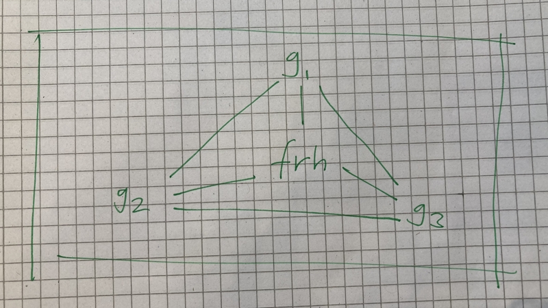
Figure: The three gladiators and Feyd-Rautha Harkonnen getting ready to fight.
⠀⠀⠀⠀⠀Next we need to tighten the conditions by requireing the Metric Space to be complete.
A complete metric space is a special kind of metric space, where every
Cauchy sequence converges to a point within the space.
Definition: Metric
Let $A$ be a nonempty set. A real-valued function $d:A x A \rightarrow \mathbf{R}$ is said to be
a metric on $A$ if it satisfies the following conditions for all $x,y,z \in A$:
$\qquad (M1) \qquad d(x,y) \geq 0$
$\qquad (M2: Axiom of Separation) \qquad d(x,y) = 0 \text{, if and only if } x = y$
$\qquad (M3: Symmetry) \qquad d(x,y) = d(y,x)$
$\qquad (M4: The Triangle Equality) \qquad d(x,z) \leq d(x,y) + d(y,z)$
Definition: Metric Space
The set $A$ endowed with a metric $d$ on $A$ is called a metric space and is denoted by $(A,d)$.
Definition: Complete Metric Space
Let $(A,d)$ be a metric space. A sequence $\{x_n\}$ of points of $A$ is said to be convergent if there is a point $u \in A$, called the limit point, such that for each $\epsilon \gt 0$, there exists an integer $N \gt 0$ such that
$$d(x_n, u) \lt \epsilon, \quad \text{for all } n \gt N.$$
Insert: image of Cauchy sequence in 2d with upper bound vs onion or eye of tornado. A metric space $(X,d)$ is complete if every Cauchy sequence has a limit that is also in $X$, that is, the limit converges to a point in the space. Let’s take a moment and define this notion.
Definition: Cauchy sequence in a Metric space
A sequence $\{x_n\}$ is said to be a Cauchy sequence if for every $\epsilon \gt 0$
there exists an integer $N$, such that for all $m,n \geq N: d(x_m, x_n) < \epsilon$.
$$\color{black}{\spadesuit}$$
Properties of a Metric Space
A Metric space has properties that we can lean on once we start trying to prove claims about how things behave in it. There are four properties that we need to be aware of:
- Non-negativity: The distance between a pair of gladiators is never less than zero (this requirement is necessary otherwise two gladiators could occupy the exact same physical space in the arena, which makes no sense.). We formalize this requirement as: $d(x,y) \geq 0$.
- Identity: The distance between a gladiator and itself is always 0, which we formalize as $d(x,y)=0 \text{ if and only if } d=y$ (which translates into: if the distance between gladiator $x$ and gladiator $y$ is zero, then they are in fact the same gladiator).
- Symmetry: The distance between gladiator A, Feyd-Rautha, and gladiator B, , is the same as the distance between B and A: $d(x,y) = d(y,x)$.
- Triangle inequality: In an arena with only 2 gladiators and 1 lion, the distance between the gladiators x and y, cannot exceed the combined distance between gladiator A and B, and gladiator B and the lion, $d(x,z) \leq d(x,y) + d(y,z)$.
Lipschitzian Maps
This post is about contraction, so let’s take a moment and make sure we understand the meaning of that word in the mathematical context at hand. A function between two metric spaces, $f:(X,d_X) \rightarrow (Y,d_Y)$ is said to be Lipschitz continuous if there exists a non-negative constant $K \geq 0$, such that for each pair of points $x_1, x_2 \in X$ we can multiply the distance between the pair $(x_1,x_2)$ in the arena $X$ with the constant $K$ and we will get a contraction of the arena with is equal in size or smaller. Formally we can write this as: $$K \cdot d_X(x_1,x_2) \geq d_Y(f(x_1),f(x_2))$$
The smallest such constant $K$, is called the Lipschitz constant of $f$. Bounded variation: Lipschitz continous functions do not oscillate wildly. Their rate of change is bounded.
We want to highlight a particular type of function that we’ll use. A function that we can apply to every point in our set, and every result from using the function will itself be a point in the arena. In other words, the function maps a set onto itself: $F: X \rightarrow X$. Now, this function is said to be Lipschitzian if there exists a constant $\alpha \geq 0$ such that:
$$d(F(x), F(y)) \leq \alpha \cdot d(x,y) \text{ for all } x,y \in X \tag{1}\label{eq1}$$
Equation $\eqref{eq1}$ is called the Global Stiffness Equestion and is the focus of this post.
Contraction Constant The constant places stronger conditions on how the distance between the combatants change. It’s not only getting smaller, it’s getting smaller by a fixed scaling constant, $k$. The smallest $\alpha$ for which $\eqref{eq1}$ holds is called the Lipschitz constant for $F$, and is given its own denotation, $L$.
Definition: A Lipschitzian mapping $T: M \rightarrow M$ with Lipschitz constant $k \le 1$ is said to be a contraction mapping.
If $L < 1$ then we say that $F$ is a contraction, basically what this means is that if we apply function $F$ to every pair $(x,y)$ in the Harkonnen Arena (the set $X$) then the entire arena will contract in size (think, we scale it down).
If, on the other hand, $L=1$ then we call $F$ a nonexpansive, meaning, we can apply the function to every pair of points$(x,y)$ in the arena, without worrying that the size of the arena will increase.
Handy Notation
Now we want to introduce notation that will simplify our discussion. Going forward we will use this nifty notation of an inductive application of a map - representing repeated application of our contraction map to a particular point $x$.
$$\begin{align} F^0(x) = x \\ F^{n+1}(x) = F(F^n(x))\end{align}$$
Let’s break this down.
$F^0(x)=x$ simply means that if we apply the function $0$ times to $x$, then we get $x$ back.
What’s next is it bit more involved, here we’re defining a recurrent function, where the result of applying the function the first time is then what we’ll use when we apply the function a second time, and so on and so on.
Let’s look at an example.
Let’s say that we have a Metric Space $(Y,d)$ where the distance between two points $x_1, x_2$ is $d(x_1,x_2)=80$.
We also have a contractive function $F$ that takes $x$, the distance between two points in the square, and cuts it in half, $F(x) = {1 \over 2}x$. If we run this function repeatedly, where each iteration gets the output of the former iteration, we get.
$F^0(80)= \text{ by power law definition} = 80$
$F^1(80)=F(F^0(80))=F(80)={1 \over 2} \cdot 80=40$
$F^2(80)=F(F^1(80))=F(40)={1 \over 2} \cdot 40=20$
$F^3(80)=F(F^2(80))=F(20)={1 \over 2} \cdot 20=10$
$F^4(80)=F(F^3(80))=F(10)={1 \over 2} \cdot 10=5$
So, we can se that by applying our halving function four consecutive times to the pair of points in our metric space, the initial distance between them, 80, is reduced to 5. A contraction.
The Banach Fixed Point Theorem
We have finally reached the finish line of this article, a mathematical result, sparkling like a jewel - The Banach Fixed Point Theorem. Also known as the Contraction Mapping Principle, or CMP for short. The theorem is remarkable in its simplicity, yet it is probably the most widely used fixed point theorem in mathematical analysis.
⠀⠀⠀⠀⠀The strength of the CMP lies in that the contractive condition on the mapping is easy to test, and the theorem only requires the structure of a complete metric space to be applicable.
We will use the same key ingredients of the CMP as it appeared in Banach’s original 1922 thesis [1].
Theorem 1.1 (Contraction Mapping Principle)
Let $(A,d)$ be a complete metric space and let $\lambda : A \rightarrow A$ be a contraction
with a Lipschitzian constant $0 \leq k \lt 1$. Then $\lambda$ has a unique fixed point $u \in A$.
Furthermore, for any $c \in A$ we have that
$$\lim_{n \to \infty}\lambda^n(c) = u$$
and for each $c \in A$,
$$d(\lambda^n(c),u) \leq {k^n \over 1-k} \cdot d(c,\lambda(c)) \tag{2}\label{eq2}$$
Proof: To prove the CMP we need to convince ourselves of two things;
- There exists a fixed point in the arena (Existence), and 2. it is the only one (Uniqueness).
⠀⠀⠀⠀⠀_Proof of Uniqueness_ ():
We start by proving that given the stated conditions of the theorem then
there can only exist one (unique) fixed point $u$ in the metric space (in our case Feyd-Rautha).
⠀⠀⠀⠀⠀Let’s say that we have two arbitrary gladiators $x$ and $y$ in the Harkonnen arena $H$.
If there’s more than one fixed point, then there has to be at lest two.
Let’s say that it’s these two gladiators $x$ and $y$.
Remember, being a fixed point means that regardless how many times we change the
size of the metric space by applying the function $F$, your position will remain the same - or, $x=F(x)$.
⠀⠀⠀⠀⠀We also need to remember that the theorem places the condition
on $F$ of being a contraction function with a Lipschitzian constant $L$. That changes everything, for starters, if $F$ is a contraction function then we know that it’s value has to be $[0,1)$, and every value that it is applied to, for
example $F(x)$ will be smaller than before.
⠀⠀⠀⠀⠀But if both $x$, and $y$ are fixed point
then the distance between them can’t change when we apply the contraction function $F$, or formally: $d(x,y) = d(F(x),F(y))$. But we also know that $L < 1$ (since
it’s a contraction), and no value multipled by another value between 0 and less than one, $[0,1)$, can do anything but decrease in size. So, $L \cdot d(x,y)$ has
to be lower than $d(x,y)$, which can only be true if $d(x,y)=0$, because it would be a contradiction if $x$ and $y$ are both fixed points in the metric space $X$ and
$L \cdot d(x,y) \geq d(x,y)$.
$$d(x,y) = d(F(x), F(y)) \leq L \cdot d(x,y) \tag{3}\label{eq3}$$
This is a contradiction because we’re supposed to be able to arbitrarily pick any two points in the metric space, and the distance between them should
decrease after each application of $F^n$.
So, by proof of contradiction, there can only be one unique fixed point, in a
complete contraction Lipschitzian metric space.
⠀⠀⠀⠀⠀If we contract the arena, for example repetedly halving it four times, and we still end up with the same distance between our two gladiators $x$ and $y$, then $x=F(x)$ and $y=F(y)$
which can only be true if the distance between them is 0, $d(x,y)=0$.
⠀⠀⠀⠀⠀Next we need to show existence of a fixed point.
We start by selecting an arbitrary Gladiator in the arena, $x \in X$.
We remind ourselves of the earlier discussion on cauchy sequences and convince ourselves that repeatedly applying our contraction function $F$ will create
a sequence of numbers. For example, in our earlier example where we had $F(x)={1 \over 2}x$
and an arena of size 80, repeatedly applying $F$ for $n \in \{0,1,2,3,4\}$ resulted in the sequence $\{80,40,20,10,5\}. \quad \square$
⠀⠀⠀⠀⠀_Proof of Existence_ (there is a fixed point combatant in the Arena): We start by reminding ourself of two important conditions that the CMP places on the Metric space. First, it has to be closed. Let’s take a moment and make sure we understand what that means. Have a look at these two
M is closed means that M contains all of it’s limit points.
And just like that, the proof of The Banach Fixed Point Theorem is done. $$\blacksquare$$
Acceptable Quality Area Below
Exercises
Theoretical knowledge is great. It’s also nice to convince ourselves that we know how to use our new knowledge. Here are three exercises1 on which we can practice our Fixed Point Theory Kung-Fu:
-
Let $F$ be a contraction created from an incomplete Metric Space into itself.
Show that it need not have a fixed point. -
Let $\bar B_r$ be a closed ball of radius $r \gt 0$, centred at zero, in a Banach space $E$, where $F : \bar B_r \rightarrow E$ is a contraction and $F(-x) = -F(x)$ for $x \in \partial \bar B_r$.
Show that $F$ has a fixed point in $\bar B_r$. -
Let $U$ be an open subset of a Banach space $E$ and let $F: U \rightarrow E$ be a contraction.
Show that $(I - F)(U)$ is open.
Hang on! Where are the answers to the exercises? Proving something is about convincing ourselves that our line of argument is correct. If we’re able to do that, then there’s no need for answers. So, work through the exercises until you are 100% convinced that your proofs are correct.
Example: Reprogramming Satellite Orbits
It’s the year 2150, Man has become a space traveling organism. Let’s say we’ve been tasked with reprogramming the orbits of a 1000 satellites orbiting a small planet in the Quadrant Solar System.
package main

import (
	"fmt"
	"gonum.org/v1/gonum/mat"
)

// Function to print a matrix
func printMatrix(matrix mat.Matrix, name string) {
	r, c := matrix.Dims()
	fmt.Printf("%s = \n", name)
	for i := 0; i < r; i++ {
		for j := 0; j < c; j++ {
			fmt.Printf("%6.2f ", matrix.At(i, j))
		}
		fmt.Println()
	}
}

func main() {
	// Step 1: Define the system Ax = b
	// A represents the linear relationship between aircraft paths
	// A is a 3x3 matrix for three aircraft
	A := mat.NewDense(3, 3, []float64{
		2, 1, 0,  // Relation between aircraft 1 and 2
		1, 2, 1,  // Relation between aircraft 2 and 3
		0, 1, 2,  // Relation between aircraft 3 and 1
	})

	// x is the vector of adjustments we want to solve for (3x1)
	// This represents adjustments in speed and altitude for each aircraft
	x := mat.NewVecDense(3, nil)

	// b represents the target adjustments we want (constraints)
	// For example, final positions or speed/altitude changes
	b := mat.NewVecDense(3, []float64{10, 5, 8})

	// Step 2: Solve the system Ax = b
	// Create a LU decomposition of A
	var lu mat.LU
	lu.Factorize(A)

	// Solve for x using the LU decomposition and the target vector b
	err := lu.SolveVecTo(x, false, b)
	if err != nil {
		fmt.Println("Error solving system:", err)
		return
	}

	// Step 3: Print results
	printMatrix(A, "Matrix A")
	fmt.Printf("Vector b = \n%v\n", mat.Formatted(b))
	fmt.Printf("Solution x (adjustments) = \n%v\n", mat.Formatted(x))

	// Interpret the solution x
	fmt.Println("Interpretation: Each value in x represents the necessary adjustments")
	fmt.Println("to the speed/altitude of the aircraft to optimize the flight paths and avoid collisions.")
}
We end up with a Matrix, $A$ A: The ballistic system’s dynamics matrix, accounting for gravity, air resistance, and projectile properties. Vector x x: The projectile’s velocity and position. Vector b b: The external forces such as gravity or air resistance.
Many problems can be reformulated to precisely ask for a fixed point of a function. A very simple example is the following:
Suppose that $A$ is an $𝑛×𝑛$ matrix, thought of as a function $𝐴:ℝ^𝑛→ℝ^𝑛$.
Solving $𝐴𝑥=𝑏$ is an extremely important problem (I hope this does not require elaboration).
Now, $𝐴𝑥=𝑏$ holds if, and only if, $𝐵𝑥=𝑥$ where $𝐵𝑥=𝑥−𝐴𝑥+𝑏$. So, here the problem of solving $𝐴𝑥=𝑏$ is transformed, via defining a new function $𝐵:ℝ^𝑛→ℝ^𝑛$, to a fixed point problem.
If you can now equip $ℝ^𝑛$ with a metric structure (for instance, one of the many norms you can place on $ℝ^𝑛$) such that $𝐵$ is a contraction, then you obtain an iterative process guaranteed to converge to the solution of the system, no matter which initial point you use to start the process.
Show the example below in code and time it: fixed point vs solve linear eq. Of course, there are precise methods to solve linear equations, but they tend to be computationally hard. The Banach Fixed Point theorem in this case is thus very useful.
Bibliography
[1]: Banach S. Sur les opérations dans les ensembles abstraits et leur application aux équations intégrales. Fundamenta Mathematicae. 1922;3:133-181
[2] Tarski A. A lattice-theoretical fixpoint theorem and its applications. Pacific Journal of Mathematics. 1955;5(2):285-309
[3] Ansari QH, Sahu DR. Fixed Point Theory and Variational Principles in Metric Spaces. Cambridge University Press; 2023.
[4] Franklin, J. N. Methods of Mathematical Economics Theory, Siam, 2002.
$$\color{red}{\diamondsuit}$$
-
These exercises were taken from page 9 in the book Fixed Point Theory and Applications by R.P. Agarwal, M. Meechan, and D. O´Regan, Cambridge University Press, 2001. ↩︎